
Introduction to Deep Learning
Introduction
If you have reached here, then I assume that you have at least heard once about Deep Learning. But actually what is it? This is the point where we lose it. Time and again we hear about the groundbreaking research being done in this field, products being built by tech giants like Google, Microsoft, Apple, Amazon and much more. What does actually go under the hood of these awesome projects?
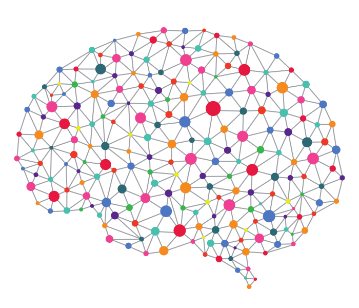
The basic underline of Deep Learning is Neural Network, not just any Neural Network but Deep Neural Network (DNN). It looks like this.
Looks frightening, isn’t it? But actually, it is not that complex to understand. A little amount of linear algebra and calculus coupled with knowledge of a programming language and we are good to go forward with it. However, prior knowledge of the mathematical stuff is not a necessary condition.
Motivation
Tech giants are competing and pushing the boundaries of technology every day and Deep Learning being the hottest field for advancement has certainly caught the eye of these blue chip companies.


Day after day revolutionary engineering has resulted in many groundbreaking technologies ranging from medical, entertainment to Gaming. These huge successes and many more to come, interests us to delve into this field. With such motivation we must continue on our journey to learn about the very foundation of this hugely popular terminology “Deep Learning”.
What are Deep Neural Networks
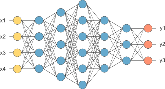
Deep Neural Networks are nothing but stacking of layers of neurons one over the other. A Neurons is a unit of Network which performs a set of computation and passes on the output to next layer where the same process is repeated again.
 As you can see in above image we have a neuron computing two components and forwarding the output to the next layer where similar computation is repeated.
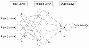
A DNN primarily consists of three components:
- Input Layer
- Hidden Layers (>=1, say L)
- Output Layer (=1)
The network collectively is called (L+1) Layer Neural Network
Each successive hidden layer is capable of computing complex features from the given input and its computation is comparatively more complex than its predecessor layers.
We also have a 1 Layer Neural Network which is also called Logistic Regression, but is not as good as compared to a DNN.
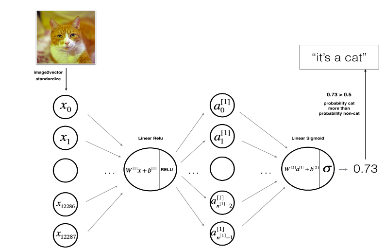
Under The Hood
The above confusing Neural Network image can be demystified in following steps:
As usual you will follow the Deep Learning methodology to build the model:
- Aquiring Dataset
- Data Preprocessing and Building Utilities.
- Build The DNN
- Initialize parameters / Define hyperparameters
- Loop for num_iterations:
a. Forward propagation
b. Compute cost function
c. Backward propagation
d. Update parameters (using parameters, and grads from backprop) - Use trained parameters to predict labels
Let’s take each step and expand upon the complete process.
We will be usnig Python as our programming language combined with numpy for our mathematical computations.
Reference can be taken from following links for any issues :
Python
Numpy
Dataset
To Demonstrate the power of Deep Neural Network we will try to Build an Image Classifier(Cat vs Non Cat). The dataset will consist of:
- Training (13 Images)
- Testing (24 Images)
On the same dataset we will compare it to one using Logistic Regression model.
Building Utilties
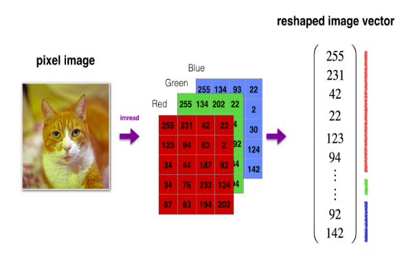
Any image cannot be directly fed into the Neural Network ans computer understands numbers. So the image must be converted into numerical form so that it can be feeded into the DNN. This conversion of Image to numerical data is called Image Vectorization.So the image has to be converted into a shape: (ht, wd, 3).
We will have m(13 in our case) training examples so final matrix shape that will be feeded as the Input Layer becomes: (m, ht, wd, 3).
A color image basically has three components.
- Height(ht)
- Width(wd)
- Color Channels(RGB = 3)
The following code snippet demonstrate the above explained process.
Load the pre-requesite dependencies
# file_name: utils.py

import os
import numpy as np
from PIL import Image
import PIL
from scipy.misc import toimage
store the path of training and testing data for future use
path1 ='path_to_training_data'
path2 ='path_to_test_data'
Components of utility are:
- image_to_arr
Takes list of all images and converts them into a (m, 64, 64, 3) matrix, special care must be taken of dimensions and datatype stored in the numpy arrays.
def image_to_arr(image_list, path):
	images_list_ = [] #list to store image data
	for image in image_list: # for each image
		im = Image.open(path + '/' + image) # open the image
		im = im.resize((64,64)) # resize the image to 64*64 shape
		im = np.array(im.getdata()).reshape(im.size[0], im.size[1], 3) # convert the digital image to numpy array
		images_list_.append(im) # store the image data to list
	images_list_ = np.asarray(images_list_) # convert the list into numpy array
	images_list_ = images_list_.astype('float32') # set the data type of array as float32
	return images_list_ # return the image data
- gen_labels
Takes the labels of the images converted to numpy arrays and genrates output labels for them (0=Non_Cat, 1= Cat). Shape of array must be (1,m).
def gen_labels(image_list, path):
	y = [] # store image labels
	for image in image_list: # for each image in the list
		if image[:3]=='cat': y.append(1) # if image_label cat store 1
		else: y.append(0) # else store 0
	y = np.asarray(y) # convert list to numpy  array
	y = y.astype('float32') # set the data tyoe to float32
	return y.reshape(1,y.shape[0]) return the label array
- load_image
Takes both functions and computes the result for training and testing images and returns the requisite numpy arrays as output.
def load_image():

	# load training/testing data
	images_train = os.listdir(path1)
	images_test = os.listdir(path2)

	# train image data and labels will be stored here
	images_train_ = image_to_arr(images_train, path1)

	## test image data will be stored here
	images_test_  = image_to_arr(images_test, path2)

	#toimage(images_train_[0]).show() # to see image back

	# load train/test labels
	y_train = gen_labels(images_train, path1)
	y_test  = gen_labels(images_test, path2)

	return images_train_, y_train, images_test_, y_test
Work not done yet!
Need to create one more utility file which contains:
Dont forget to import numpy
# file_name: L_DNN_utils.py

import numpy as np
- sigmoid_activation: The forward activation function for the Output layer.
def sigmoid(Z):
	# input:
	# Z: linear computation of each layer neurons
	# output:
	# A: each layer activation
	# Z: linear computation for storing pursposes

	A = 1/(1+np.exp(-Z)) # for more information regarding formula refer to Activation section below
	return A, Z
- relu_activation: The forward activation function for hidden layers.
def  relu(Z):
	# input:
	# Z: linear computation of each layer neurons
	# output:
	# A: each layer activation
	# Z: linear computation for storing pursposes

	A = np.maximum(0,Z) # for more information regarding formula refer to Activation section below
	return A, Z
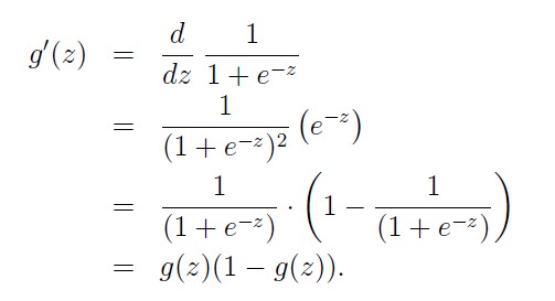
- sigmoid_derivative: The derivative of sigmoid function for backpropagation.
def sigmoid_derivative(dA, activation_cache):
	# input:
	# dA: current layer activation derivative from backpropagation
	# activation_cache: current layer linear computation (Z)
	# output:
	# dZ: current layer linear computation derivative

	Z = activation_cache
	g = 1/(1+np.exp(-Z))
	dZ = dA * g * (1-g) # # for more information regarding formula refer to Activation section below
	assert (dZ.shape == activation_cache.shape) # type checking
	return dZ
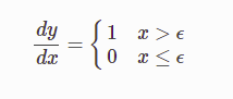
- relu_derivative : The derivative of relu function for backpropagation.
def relu_derivative(dA, activation_cache):
	# input:
	# dA: current layer activation derivative from backpropagation
	# activation_cache: current layer linear computation (Z)
	# output:
	# dZ: current layer linear computation derivative

	Z = activation_cache
	dZ = np.array(dA, copy=True)
	dZ[Z<=0] = 0 # this is the derivative step...for more info refer to Activatin section below
	assert (dZ.shape == Z.shape)
	return dZ
Data Preprocessing
The data that we work with is loaded using the Utility we built in previous step. But, furthermore preprocessing is needed before we include it in our computation. To achieve fast computation results we will use a process called Vectorization using numpy. Data preprocessing is a necessary step for that.
Steps involved in preprocessing are:
- Array Flattening: Converting input data shape from (m, ht, wd, 3 ) to (ht * wd * 3, m)
- Data Standardization: Dividing every value in matrix from 255 (255 being the max value in the input matrix)
Building the Deep Neural Network
A Deep Neural Network has following components.
Inputs (X): The input matrix provided to the DNN as training and testing datasets.
Hidden Layers: Each hidden layer is given a task to compute Forward Propagation variables
- Z (WTX + b): In this step we compute linear outputs corresponding to X but combine
it with W(weights assignmed to each Hidden Layer) with an added bias value b. - A ( g(Z) ): In this step we compute activations for our computed linear outputs so as
to obtain some non-linearity in our learning (This is an important aspect of Neural Networks).
Output Layer: The output layer is responsible to compute the final output values ( 0/1 ).
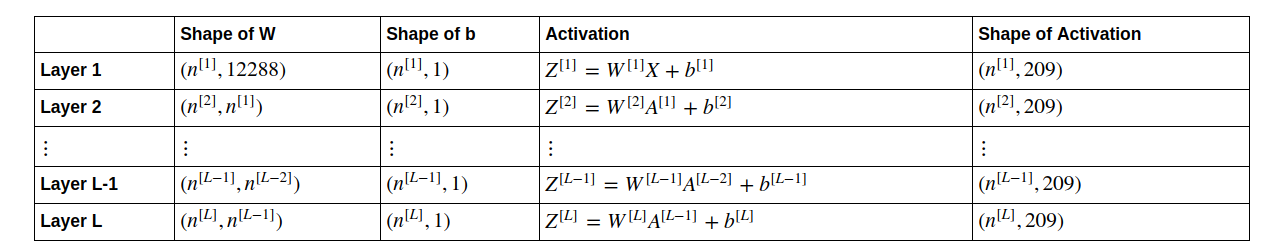
Dimensions: A lot of care must go into keeping a check on the dimensional integrity of the variables and matrices we are computing. Below is a quick guide to for what the dimensions of these computations must be.
Activations
Activations are functions that must be applied to computed linear variables (Z) so as to obtain non-linearity.
Why non-linearity ? It helps the neural network compute interesting features. Linear hidden layers are useless.
Types of activations that we use in our DNN are:
Sigmoid
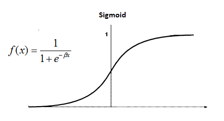
One of the famous activation functions. MUST BE USED IN OUTPUT LAYER
ReLU
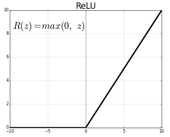
Also called rectified Linear Unit. To calculate interesting features MUST BE USED IN HIDDEN LAYERS.
Note: We also ned to calculate derivatives of these activation functions, as follows:
sigmoid derivative
relu_derivative
Componenents of DNN model
For constructing the DNN model do not forget to load these dependencies
#file_name: L_Layer_model.py

import numpy as np
import matplotlib.pyplot as plt
from L_DNN_utils import sigmoid, relu, sigmoid_derivative, relu_derivative
Initialize Parameters
The main components of the Network are the parameters which will govern the performance and learning from data. These parameters are the inputs to a neuron which facilitate the formation output. However there initialisation is a bit different from each other. These components include:
Weights(W)
Initialized as a random array of dimensions (n[L], n[L-1]) –> see dimensions image above for consultance. This random initialisation is due to the fact that if weights are initialized to 0 or some fixed value then all the neurons in same layer will be computing same values for features with no improvements which will result in symmetric Network(undesirable).
Bias(b)
Initialized as a numpy array of zeros (n[L],1).
The following can be implemented in python as follows
def init_parameters_L(layer_dims):
	# layer_dims will contain each neural network layer size, enabling us to corectly assigning dimensions to parameters

	np.random.seed(1)
	parameters = {} # create a dictinary to store the parameters
	for l in xrange(1,len(layer_dims)): # for each layer
		parameters['W'+str(l)] = np.random.randn(layer_dims[l], layer_dims[l-1])*0.01 # random initialization of Weights array
		parameters['b'+str(l)] = np.zeros((layer_dims[l],1)) # bias initialization to array of 0s

		assert(parameters['W'+str(l)].shape == (layer_dims[l],layer_dims[l-1]))
		assert(parameters['b'+str(l)].shape == (layer_dims[l],1))
	return parameters
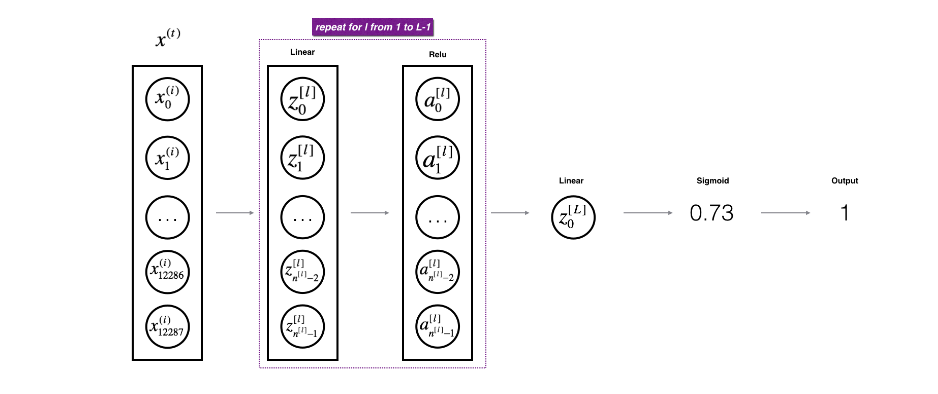
Structure of our Neural Network
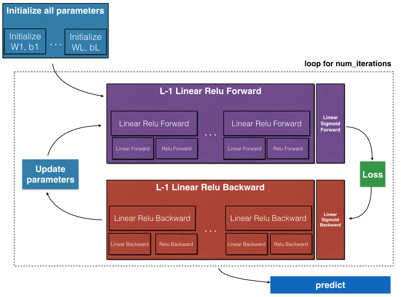
The image above demonstrates the exact structure that we are going to implement.
- We will have in total L layers in our DNN and out of these L-1 will be hidden layers.
- An outermost loop will run for num_iteration times which is as per user requirements.
- First L-1 layers will compute forward propagation variables and store them in cache for future use. We will use ReLU activation in this layer.
- Last layer will compute the same variables but activation used in this layer will be sigmoid.
- The output of last layer(L) will be used to compute loss of our model. This loss will help us initiate the backpropagation mechanism.
- The backpropagation will take help of utilities built earlier and caches maintained during forward propagation to compute the gradients necessary for tuning our model parameters.
- The gradients computed via backpropagation will be used to update our parameters.
- Running above propagation steps will enable proper tuning of parameters which can then be used in prediction of output on test data.
Forward Propagation
The first step step is to propagate inside our neural network skeleton built by initialising the parameeters mentioned above. In this step we compute the forward linear function(Z) for each neuron and their respective activations(A).
- Z = WT.A_prev + b
- A = g(Z)
g being the applied activation function on Z.
T denotes transpose.
A_prev denotes previous layer activation values (Note: for first hidden layer 1 A_prev = input(X) )
We will construct two functions:
- forward_prop_L: In this function we will compute forward linear variable(Z) and also return input parameters(A_prev, W, b) as cache.
def forward_prop_L(A_prev, W, b):
	# input:
	# A_prev: previous layer activation
	# W: current layer weights
	# b: current layer bias
	# output:
	# A: current layer activation
	# cache: containing A_prev, W, b

 	Z = np.dot(W, A_prev) + b
	assert(Z.shape == (W.shape[0], A_prev.shape[1]))
	cache = (A_prev, W, b)
	return Z, cache
- activation_forward_L: In this function we will compute Z via forward_prop_L and activations using utilities we built earlier. Return input parameters and Z as cache
def activation_forward_L(A_prev, W, b, activation):
	# input:
	# A_prev: previous layer activation
	# W: current layer weights
	# b: current layer bias
	# activation: Relu pr sigmoid (depends on the layer you are working on)
	# output:
	# A: current layer activation
	# caches: a tuple of (A_prev, W, b), Z

	if activation == "relu":
		Z, linear_cache     = forward_prop_L(A_prev, W, b)
		A, activation_cache = relu(Z)

	if activation == "sigmoid":
		Z, linear_cache     = forward_prop_L(A_prev, W, b)
		A, activation_cache = sigmoid(Z)

	assert(A.shape == (W.shape[0], A_prev.shape[1]))
	return A, (linear_cache, activation_cache)
The complete forward propagation functionality implementation after we have built the functions mentioned above will look like this.
def L_model_forward(X, parameters):
	# for first L-1 layers relu activation will be used
	# for last layer sigmoid activation will be used
	# input:
	# parameters: dictionary of W, b values of each layer(0...L)
	# X: input data
	# output:
	# AL : the output value of the last/output layer
	# caches: a list of caches returned by activation_forward_L for each layer

	L = len(parameters)//2
	A = X
	caches = [] # to store all necessary (linear_cache, activation_cache ) for backprop
	for l in xrange(1, L):
		A_prev = A
		A, cache = activation_forward_L(A_prev, parameters['W'+str(l)], parameters['b'+str(l)], activation='relu')
		caches.append(cache)
	AL, cache = activation_forward_L(A, parameters['W'+str(L)], parameters['b'+str(L)], activation='sigmoid')
	caches.append(cache)

	assert(AL.shape == (1, X.shape[1]))
	return AL, caches
Cost Function
For any model you build keeping track of the cost and minimisation of it are two important features. Cost should decrease so that it is ensured that our learning is improved with each new training sample.
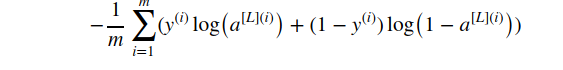
Following is the python implementation for the Cost function:
def compute_cost(AL, Y):
	#input:
	# AL: output of the last/output layer (probablistic values of model)
	# Y: train/test labels for the same
	# output:
	# cost for the outputs generated during current iteration

	m = Y.shape[1]
	cost = np.squeeze( -np.sum(Y*np.log(AL) + (1-Y)*np.log(1-AL))/m ) # [[val]] = val using squeeze
	assert (cost.shape == () )
	return cost
Backpropagation
The most important or we can say the heart of the model is this step. In this step we compute the gradients of each paramter used in our computation. In simpler words we try to calculate the measure of the effect that a parameter has on the Loss function. In mathematical terms we use a method called chaining rule in calculus combined with derivatives to calculate all the derivatives. But without delving into the complicated maths of it, below are the formulae we need to compute.
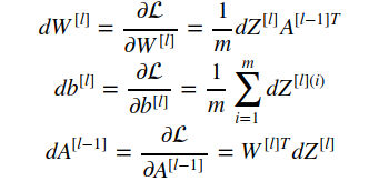
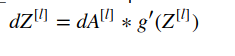
Following is the python implementation of the above mentioned formulae.
The following function will compute dA[l-1], dW[l], db[l] where l is the layer for which gradients are being computed:
def backprop_L(dZ, cache):
	# input:
	# dZ: current layer linear computation derivative
	# cache: a tuple containing A_prev, W, b
	# output:
	# dA_prev: previous layer activation derivative
	# dW: current layer weights derivative
	# db: currrent layer bias derivative

	A_prev, W, b = cache
	m = A_prev.shape[1]

	dW = np.dot(dZ, A_prev.T)/m
	db = np.sum(dZ, axis=1, keepdims=True)/m
	dA_prev = np.dot(W.T, dZ)

	assert( dW.shape == W.shape)
	assert( db.shape == b.shape)
	assert( dA_prev.shape == A_prev.shape)

	return dA_prev, dW, db
def activation_backward_L(dA, cache, activation):
	# input:
	# dA: current layer activation derivative
	# cache: a tuple containing A_prev, W, b
	# activation: current layer activation (ReLU / sigmoid)
	# output:
	# dA_prev: previous layer activation derivative
	# dW: current layer weights derivative
	# db: currrent layer bias derivative

	linear_cache, activation_cache = cache
	m = linear_cache[0].shape[1]
	if activation == 'relu':
		dZ = relu_derivative(dA, activation_cache)
		dA_prev, dW, db = backprop_L(dZ, linear_cache)
	if activation == 'sigmoid':
		dZ = sigmoid_derivative(dA, activation_cache)
		dA_prev, dW, db = backprop_L(dZ, linear_cache)

	return dA_prev, dW, db
On combining both the functions we will get the following backprop model:
def L_model_backward(AL, Y, caches):
	# input:
	# AL: Last layer activation values
	# Y : train/ test labels
	# caches: list of every layer caches containing A_prev, W, b, Z
	# output:
	# grads: dictionary of the gradient/ derivative values for parameters for each layer

	Y = Y.reshape(AL.shape)
	dAL = -(np.divide(Y, AL) - np.divide(1-Y, 1-AL))
	L = len(caches)
	grads = {}
	m = AL.shape[1]

	# for the only sigmoid layer
	current_cache = caches[L-1]
	grads['dA'+str(L)], grads['dW'+str(L)], grads['db'+str(L)]  = activation_backward_L(dAL, current_cache, activation='sigmoid')

	#for the relu layers
	for l in xrange(L-2,-1,-1):
		current_cache = caches[l]
		grads['dA'+str(l+1)], grads['dW'+str(l+1)], grads['db'+str(l+1)] = activation_backward_L(grads['dA'+str(l+2)], current_cache, activation='relu')

	return grads
These gradients are used in the updation process.
Updating Parameters
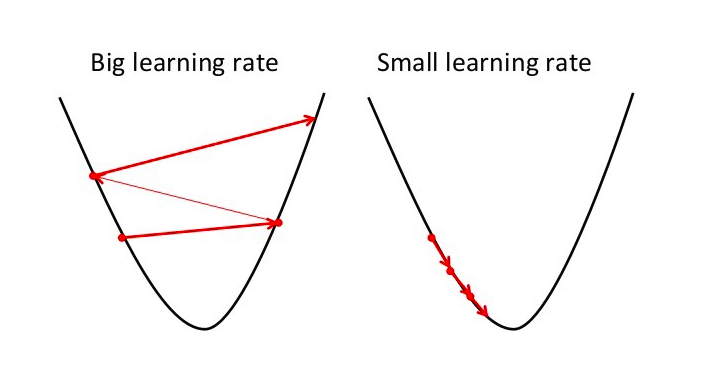
After computing the gradients for the parameters we need to update the parameters using the gradients and learning rate which is set by the user. Now user has to be careful while chosing a learning because if learning rate is high then our algorithm will overshoot and miss the global minima while minimizing the loss. A small learning rate will ensure progress towards the minima slowly but wont overshoot it.
After we have selected a learning rate its time to update our parameters. The formulae for doing so are shown below:
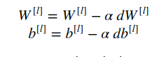
The following python implementation demostrate the updation process:
def update_parameters(parameters, grads, learning_rate):
	# input:
	# parmeters: dictionary containing weights, biases for each layer
	# grads: dictionary of gradients computed via backprop for parameters of each layer
	# learning_rate: the learning_rate enabling us to update our parameters
	# output:
	# parameters: updated dictionary of parameters

	L = len(parameters)//2 # total number of layers in our model
	for l in xrange(1,L+1): # for each layer 1...N
		parameters['W'+str(l)] -= learning_rate * grads['dW'+str(l)]
		parameters['b'+str(l)] -= learning_rate * grads['db'+str(l)]

	return parameters
Evaluation
To check how well our model performed we need to evaluate it. Output layer computes the activations using Sigmoid function. The probablistic values computed can be converting into binary outputs using a threshold (=0.5) set by the user.
To evaluate the model following python implementation of prediction is done:
def predict(X, y, parameters):
	# input:
	# X: train/ test input data
	# y: train/test labels
	# parameters: the learned parameter inputs for evaluation
	# output:
	# p: probablistic values of output layer based on a threshold(=0.5 here)

	m = X.shape[1]
	n = len(parameters)//2

	# forward prop
	probas, caches = L_model_forward(X, parameters)
	p = (probas > 0.5).astype(int)
	print "Accuracy: " + str(np.sum(p==y)/float(m))
	return p
Image Classification using Deep Neural Network
Load the requisite utilities
# Jupyter Notebook

import numpy as np
import matplotlib.pyplot as plt
from L_Layer_model import *
import scipy
from PIL import Image
from scipy import ndimage
from utils import *


%matplotlib inline
plt.rcParams['figure.figsize'] = (5.0, 4.0) # set default size of plots
plt.rcParams['image.interpolation'] = 'nearest'
plt.rcParams['image.cmap'] = 'gray'

%load_ext autoreload
%autoreload 2

np.random.seed(1)
Load the dataset
train_x_orig, train_y, test_x_orig, test_y = load_image()
Convert the training dataset into required dimensions and standardize the train/test input data.
# Reshape the training and test examples
train_x_flatten = train_x_orig.reshape(train_x_orig.shape[0], -1).T   # The "-1" makes reshape flatten the remaining dimensions
test_x_flatten = test_x_orig.reshape(test_x_orig.shape[0], -1).T

# Standardize data to have feature values between 0 and 1.
train_x = train_x_flatten/255.
test_x = test_x_flatten/255.

print ("train_x's shape: " + str(train_x.shape))
print ("test_x's shape: " + str(test_x.shape))

'''
output:

train_x's shape: (12288, 13)
test_x's shape: (12288, 24)
Build the L-layer Neural Network (Here for demonstration we build a 5 layer Model - check layer_dims )
Start by initializing the layer dimensions
## mention how many layer network you want here by adding layer dimensions in layer_dims

layers_dims = [12288, 20, 7, 5, 1] # we are going for a 5-Layer Deep Neural Network
Following code enables us to construct a Deep Neural Network for our corresponding layers_dims
def L_layer_model(X, Y, layers_dims, learning_rate = 0.0075, num_iterations = 3000, print_cost=False):
    # input:
    # X: input train/test data
    # Y: input train/test labels
    # layers_dims: a list of each layer dimensions
    # learning_rate: a value crucial for updating our parameters (W, b) after backpropagation
    # num_iterations: the total number of iterations for which we will run our model to learn parameters fit enough to predict image labels
    # print_cost: a verbose parameter for checking training status by printing cost
    # output:
    # parameters: return the parameters once the training is completed for test data evaluation

    np.random.seed(1)
    costs = [] # keep track of cost

    # Parameters initialization.
    parameters = init_parameters_L(layers_dims)
    # Loop (gradient descent)
    for i in range(0, num_iterations):

        # Forward propagation: [LINEAR -> RELU]*(L-1) -> LINEAR -> SIGMOID.
        AL, caches = L_model_forward(X, parameters)

        # Compute cost.
        cost = compute_cost(AL, Y)

        # Backward propagation.
        grads = L_model_backward(AL, Y, caches)

        # Update parameters.
        parameters = update_parameters(parameters, grads, learning_rate)

        # Print the cost every 100 training example
        if print_cost and i % 100 == 0:
            print ("Cost after iteration %i: %f" %(i, cost))
        if print_cost and i % 100 == 0:
            costs.append(cost)

    # plot the cost
    plt.plot(np.squeeze(costs))
    plt.ylabel('cost')
    plt.xlabel('iterations (per tens)')
    plt.title("Learning rate =" + str(learning_rate))
    plt.show()

    return parameters
Training time! for our model
Obtained parameters from the training will be used for testing evaluation. Take a look at the parameters being used in Model training.
parameters = L_layer_model(train_x, train_y, layers_dims, num_iterations = 2500, print_cost = True)
We can have a look at the training process
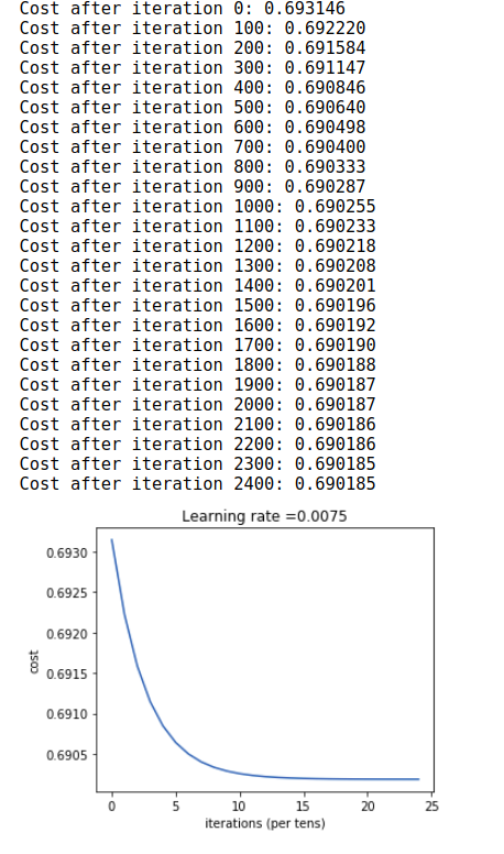
Time for evaluation on test dataset
pred_train = predict(train_x, train_y, parameters)
pred_test = predict(test_x, test_y, parameters)
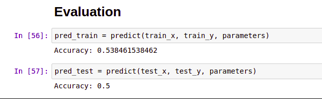
50% accuracy. Not bad! for a small dataset we used for training and testing. With bigger dataset we will certainly get higher accuracy values.
References
CS231N
deeplearning.ai
Google
All the code snippets mentioned above have been compiled as code on link given below
Introduction to Deeplearning
Have fun!
Keep Learning
Don’t forget to fork and star :P